by RC Jenkins (see previous guest posts)
Color science is an art.
And we’ve been getting a lot of crayons lately. And not the stupid ones in the 4-pack from some kid’s party that are basically just plastic and break. The good ones that just smear colors onto the page.
The biggest headline feature of the ZR is probably R3D NE (raw video format); but nobody actually cares about the technical format. It might even be pretty much the same as .NEV. What really differentiates it from .NEV is the color science that it contains. (But what exactly does this mean…? That was rhetorical.)
And not long before that, Nikon started rolling out “Flexible Picture Controls.” And before that, were the Advanced Picture Controls, which were themselves more advanced than the regular Picture Controls.
And during all of this, we had the fanboys bashing Sony’s colors or praising Fuji’s ‘Film Simulations’ and Canon’s colors. Which is always tinted a bit ironic when the same people brag about shooting raw and editing in Lightroom. But that’s a different topic. Or is it…? Hmmm…
You can’t paint without laying down some primer. So let’s put down a quick layer of primer on the raw material. What are raws?
Raws are a (lowercase) type of image file. Each photosite (~pixel) on almost all sensors can only measure an amount of light–it cannot measure the color of that light, the direction of that light, etc. Think about that. Critical thinkers will start to form a picture of the implications: ‘So if our sensor’s photosites can only measure the amount of light, doesn’t that make them black-and-white only?’
Yes, it does. We have black-and-white sensors. And our raws are black-and-white images. huhhh?
The “raw meat” is the linear value that each pixel recorded; and it’s usually 12- or 14- bits. Which means a precision of either 4096 or 16384 shades of grey, per pixel. This is better than 50 Shades of Grey. I was obligated to add this dated and irrelevant reference somewhere.
But that’s about it. Each pixel from a grid of pixels measures an amount of light. Using the photoelectric effect. (Essentially, as light hits a pixel, it builds up a charge. The pixel circuitry measures this and stores it as a digital value).
On a 24MP camera, you’ve got 24 million pixels, each with a different amount of light. And when you plot that out–where each pixel was and how dark it was–you get a black-and-white image. And that’s really the meat of the raw.
While we’re on the titillating subject of black-and-white linear tonal values, we’ll need a quick detour. There appears to be a log in the road. So pop a squat, drop the kids off at the pool, and let’s dump some info on a little thing called logs.
Log (a log gamma curve, if you’re nasty…and you are) is a tonal compression method, used to improve data efficiency in times of limited data bandwidth. Its purpose is the same as a zip file or an mp3: to get information across using less data.
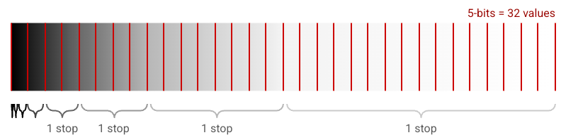
As a reference, let’s look at a quick example of a gradient from black to white. Going back to raws, remember that this is the only thing that each pixel on a sensor can measure: a quantized value of where along this dark-to-light gradient you are.
In this example, each quantized value (in red) represents a value stored in 5-bits (happened to be convenient to visualize). And across the bottom, you’ll see labels for the “stops” of light. This is the same scale as f-stops.
A few things to take note of:
And you’ll quickly see a mismatch. Remember again the earlier raw reference to linear sensor readouts? What you’ll note is that while the sensors are linear, the way we use light and stops is not. And so the issue becomes that your brighter highlights get twice as much precision as the darkest shadows. In other words, the brightest single stop gets 16 (out of the 32) digital values. The darkest stop gets just 1 distinct value (out of 32).
In a raw readout, this is all you get, and you cannot get more precise than the physical sensor gets you. Which is ok, since in real life, a 12- or 14- bit raw might give you thousands of times more precision in the highlights than in the shadows. That’s a lot; and noise will get you before a lack of digital precision. So to everyone who is like “we need 16-bit raws or Nikon will go out of business” in the comments, no you don’t.
But what if you’re shooting video instead of stills? Now you have to do tens of frames per second, for multiple minutes. Thousands of frames; and you might have a bandwidth or a file size problem. And since your output file and display is probably going to be 8-bit anyway, you can just record 8-bit. Which is fine; but doing so doesn’t always give you a lot of room to boost the darkest shadows without the risk of posterization (where you see blocks or bands of just one color suddenly changing to a slightly different color). Because (again) the shadows don’t get as much digital precision.
So what if you found a middle ground? In video, the sensor reads at 12-bits. You’re outputting and displaying (after color grading) in 8-bits. So what if you had the bandwidth and memory to record 10-bits? This might be fine. You’ve increased the precision by a factor of 4 across the board (including shadows); but what if you could be smart and do even more?
This is where log comes into play.
A log workflow is optimized for when you have 3 distinct bit depths, such as:
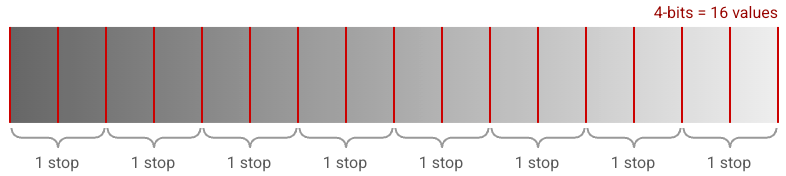
And the way it works is that the camera renders the shadows brighter (between the 12-bit read and the 10-bit file), in order to give them more bits. Log profiles will move shadows to a brighter area where they’ll get more bits. And this is fine because our cameras today have a lot of dynamic range and relatively clean shadows. But those limited bits don’t come for free–they have to come from somewhere. And so they come from the highlights. In other words, a log render of the above gradient might look more like this:
In this example, the shadows are brighter; and the stops are more evenly spread out, to provide more precision for shadows at the expense of precision in the highlights. In other words, log is lossy tonal compression, in order to improve shadow precision, at the expense of highlight precision. You’re squeezing your dynamic range to improve shadow precision. (This is, btw, also why log usually starts at ISO 800 instead of 100, even though it’s the same ‘raw ISO’: digital ISO is essentially just an output brightening factor defining the rendered (not raw) middle grey, relative to a physical amount of light captured by the sensor…but this is another topic).
The gamma (tonal) curve used to move the data bits from highlights to shadows is a logarithmic curve. Each manufacturer will make their own; they usually add the first letter of their brand to the beginning (because they’re so creative); and you can usually find technical info on these. Like Nikon’s N-Log here. (Sony’s is S-log, Canon’s is C-log, Panasonic’s is obviously V-log, etc). You can even make your own in some cases (and we’ll get to this).
But that looks blah. How do we make it look good? When we color grade (and go from 10-bits to 8-bits), we can just darken the shadows and brighten the highlights again. And if we’re lazy, we can start with a LUT (look up table), which is basically a predefined counterbalance to the log. We previously squeezed the dynamic range; and LUTs will stretch it back out. Manufacturers will usually make several different log profiles and several different LUTs. These all serve the same purpose; and they all have strengths and weaknesses, since log is (by nature) a compromise. Some do “better” in some circumstances at shadows, or highlights, or whatever.
(But if we’re just using the LUT as is, then we should really question why we’re shooting log in the first place–we could have just skipped that step altogether and had our cameras do that 12-bit to 8-bit conversion for us to get us as close to the end point as possible; or even a 12-bit to 10-bit conversion that gets us close and also gives us lots of room to grade too).
^ That’s what a log gamma curve does. And it’s most effective when you go from a higher bit depth to a lower bit depth, with an intermediate bit-depth in-between. Like a 12-bit raw to a 10-bit log to an 8-bit output. It’s not perfect–it’s specifically to reduce shadow posterization at the (minor) expense of highlight precision.
And it has less to do with color and more to do with tonal compression. Which means while log may do dynamic range well–maybe even comparable to raw in practice much of the time–it doesn’t necessarily do things like white balance or color precision as well. (But shhh…that’s later…we’re still black & white).
But this brings me to another point: as bandwidths and compression efficiencies have increased, I think log may eventually get flushed away, in favor of raw video. Maybe. Because raw doesn’t compromise like log does. Log can sometimes be added as metadata to a raw; but this is usually just for workflow consistency, like reusing LUTs.
Sooo…we’re still black and white. And gray. Where does the color come from?
Back to the physical sensors: There is a color filter above each photosite: usually either red, green, or blue. So when light passes through the filter, only some of it makes it to the other side to be measured by the (black & white) photosite. For example, if red light encounters a red filter, it will pass through and the photosite will measure a high value (“white”). If red light encounters a blue filter, it will be absorbed and no light will make it through; and the photosite will measure a low value (“black”). So each pixel is blocking certain colors, letting other colors through, and recording a black and white value. What does this have to do with anything?
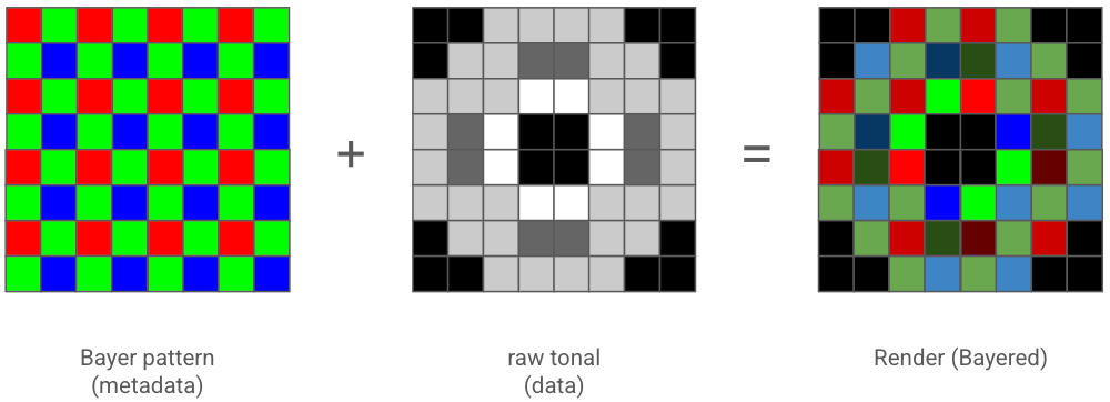
This is metadata; and it supplements the raw tonal data. So if you know that for that given sensor:
This is just a fixed pattern; and it doesn’t change shot-to-shot on a given camera. So this can be static metadata attached to the raw. Better yet: if you additionally also know the response of how red, how green, how blue each filter was (which can be different for each camera but not for each picture within that camera), then you can combine this even more precise static metadata with the actual dynamic (image-specific) black-and-white raw data that you recorded. This is enough data to inform the color processing.
And so now, we have recreated an image, where every other pixel is green; and red and blue alternate in-between these. Basically, black-and-white image with a Bayer pattern overlaid. A picture is worth 1000 words, so:
Also note that this has implications:
The important part: this last point is where a lot of the color science happens. And this is often why different raw processors using the same file might end up with different renders. And also the color science work different raw processors might perform to come up with the same renders from different raw files.
But that’s still not the color we are expecting. So on to de-bayering.
Debayering is looking at nearby pixels to guess which color that pixel should be. For example, if you have a lot of bright red and green pixels in the same area; but all of the blue pixels in that same area are dark, then chances are, the object was yellow. So you keep and use the raw tonal value (the black & white value) of the pixel as is; but you overlay yellow. Or perhaps the red was brighter than the greens, so you overlay a more ‘reddish yellow’ / orange. Etc.
Given all of the above, let’s look at a hypothetical example: Imagine that the Z8 had stronger RGB filters and was worse with dynamic range; and the Z6 had weaker RGB filters but was better with dynamic range–Nikon might apply a different tone curve and increase the color saturation between the raw and JPEG for the Z6 when producing an output. They may also try to more quickly separate red from orange from yellow, basically amplifying the sensitivity to color shifts. This path between a starting point and a render is essentially the color science.
My guess is that the R3D NE (raw video files) announced alongside the Nikon ZR are actually not a fundamental change to nraw. I think instead, it is mainly a marketing gimmick–however, it’s one with something useful underneath. I think Nikon has worked with RED to tweak the “color science” metadata in the path between the raw tonal data–which I believe will be the same as the Z6iii’s–and the rendered images. Along the lines of the “what is the red color frequency response / filter strength” -type metadata. And that as such, one could create a LUT or color corrections to match a Z6iii to a ZR to RED, since raw is raw. It would just be more work between the raw and the (consistent) render.
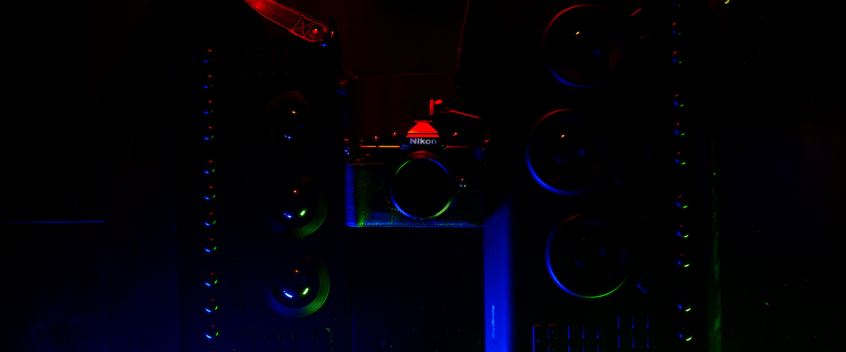
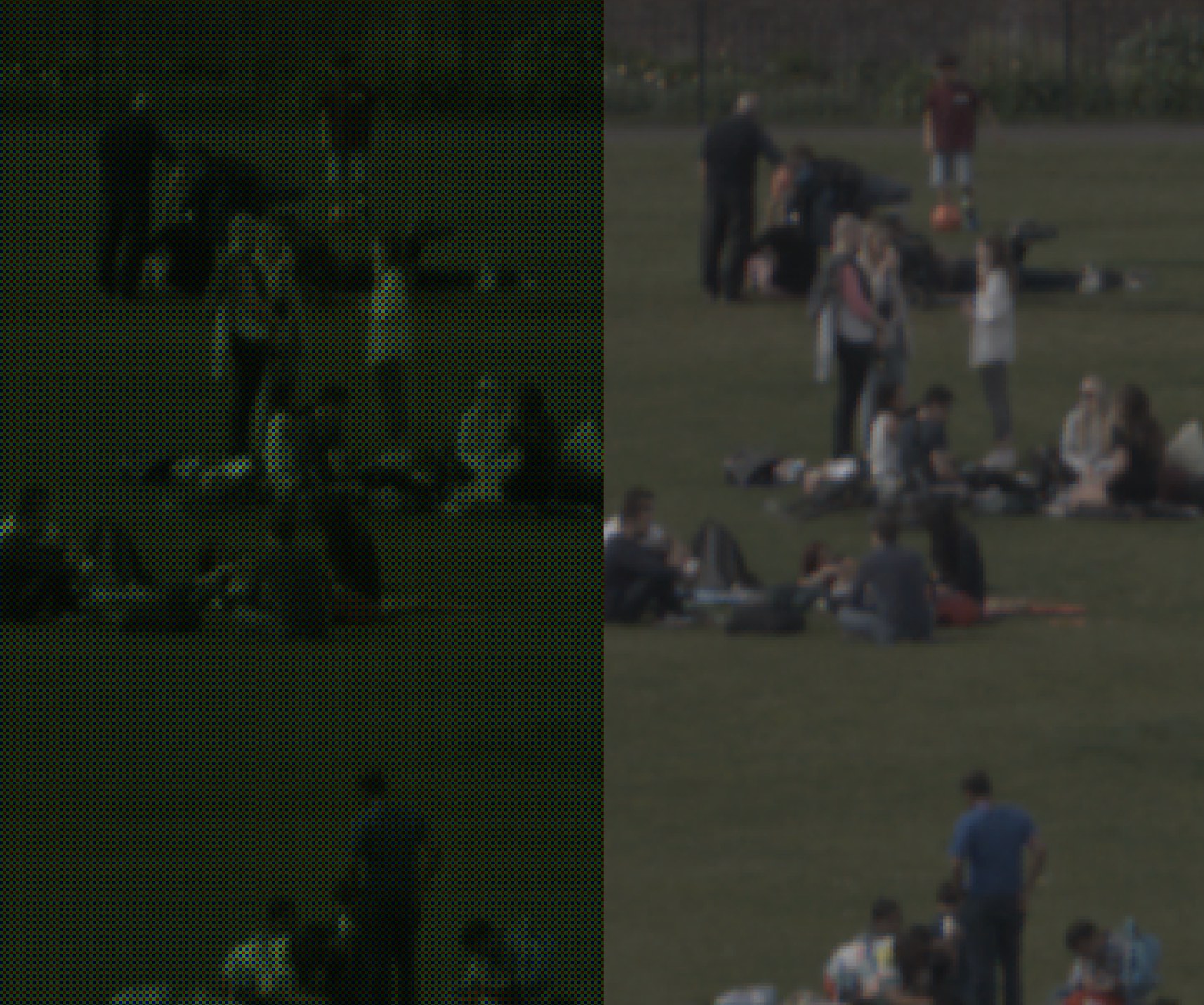
Anyway, let’s close this out with a very tight crop of the raw (with bayer overlay) on the left; and a rendered color image on the right. These are based (I believe) on more generic renders in RawDigger, rather than how Nikon might apply its color science.
(BTW, it was near impossible to find a real image to make this point, where I could zoom in so tight to display individual pixels, while also being intuitive as to reference what we’re looking at, with some varying colors and contrast, from some of these cameras! Our resolutions are ridiculous…and this was from a Z6 because the Z8 was even tougher).
Anyway: now, we’ve arrived at a color photo. But we can also see some of the nuance when it comes to color; and we can keep that in mind as we move on from the primer. Yes, all of that was just a primer.
So let’s FINALLY stop talking about the science and instead talk about the fun artsy part that I really wanted to talk about: flexible picture controls yaaay! Flexible picture controls are basically awesome. And it’s where you can artistically nerd out on your own color science experiments.
First: what are picture controls? I have no idea why I’m asking myself that. I suppose to stage the response? I have a feeling I’m going to be doing a lot of these “question? answer” -type statements coming up.
Picture controls are Nikon’s rendering engine from the 12- or 14- raws to an 8- or 10- bit output (like a JPEG). The picture controls operate at a 16-bit precision (reference) between the raw and rendered image. They are the color science.
And they are now so powerful. They are brilliant if you want to just enjoy shooting without all of the manual editing later. I tend to use these more for casual, fun shooting like when I’m out with friends and we just want to snapbridge to the phone and post them; but I’ve recently been doing more pro stuff with them too. And I’ve always also used them in weird ways to really push the boundaries of the cameras.
Let’s walk through why they are so awesome. And maybe even a bit of evolution, and even why I think Nikon are industry leaders here and even put Fuji’s film simulations to shame.
Since the earliest few versions around 20 years ago (?), Nikon has allowed us to do tone curve adjustments. Sound familiar? Remember how we talked earlier about how log curves work? Yes, this means we can create our own log gamma curves, and have been able to do this for years. In fact, when the Z6 first came out in 2018 and people were complaining it didn’t have log while Sony’s A7iii did–this was incorrect. Sony had a built-in / preloaded 8-bit log in the A7iii. But we could create our own 8-bit logs in the Z6/Z7. You may have even seen some out there, like “BeatLog.” Yes, these were only 8-bit; but remember how tonal precision works when you darken shadows (and these were usually plenty). And now that we’ve got 10-bit h.265 recording, we’ve got 10-bit logs as well (in addition to nlog).
But another creative way we can use tone curve adjustments is to “zoom in” to various parts of the dynamic range. Want to ETTR and find the precise point your sensor starts clipping what’s important in the raw? Make a steep tone curve in the highlights, use this to get your exposure settings, and then switch back to a different picture control to take the shot. Want to see what your shadows look like and if you need to stack for HDR? Do the opposite–make a steep tone curve in the shadows. Want to see both at the same time in your viewfinder, because you’re deathly afraid of clipping highlights? Make a combination of a log and sharp ceiling. These are essentially an advanced metering technique for precision exposures.
Later (around 10-15 years ago?), Nikon made some advancements to the picture controls, adding things like d-lighting, clarity, mid range sharpening, etc. Essentially, these were various localized tonal corrections, where they compare tonal values of nearby pixels. And these were great.
But that stuff is not fun. And while I liked them, I always had a problem with them: these were always just tonal corrections. They really only dealt with the black-and-white parts of the image and not the actual color science.
But that has finally changed with flexible picture controls. Flexible picture controls allow more control over actual color corrections, and not just tonal control. You can make oranges redder or yellower; you can make shadows bluer and highlights yellower. You can make greens look less saturated and neon. You can make purples darker but more saturated. It’s pretty amazing. And frankly, they make Fuji’s film simulations look so basic and limited.
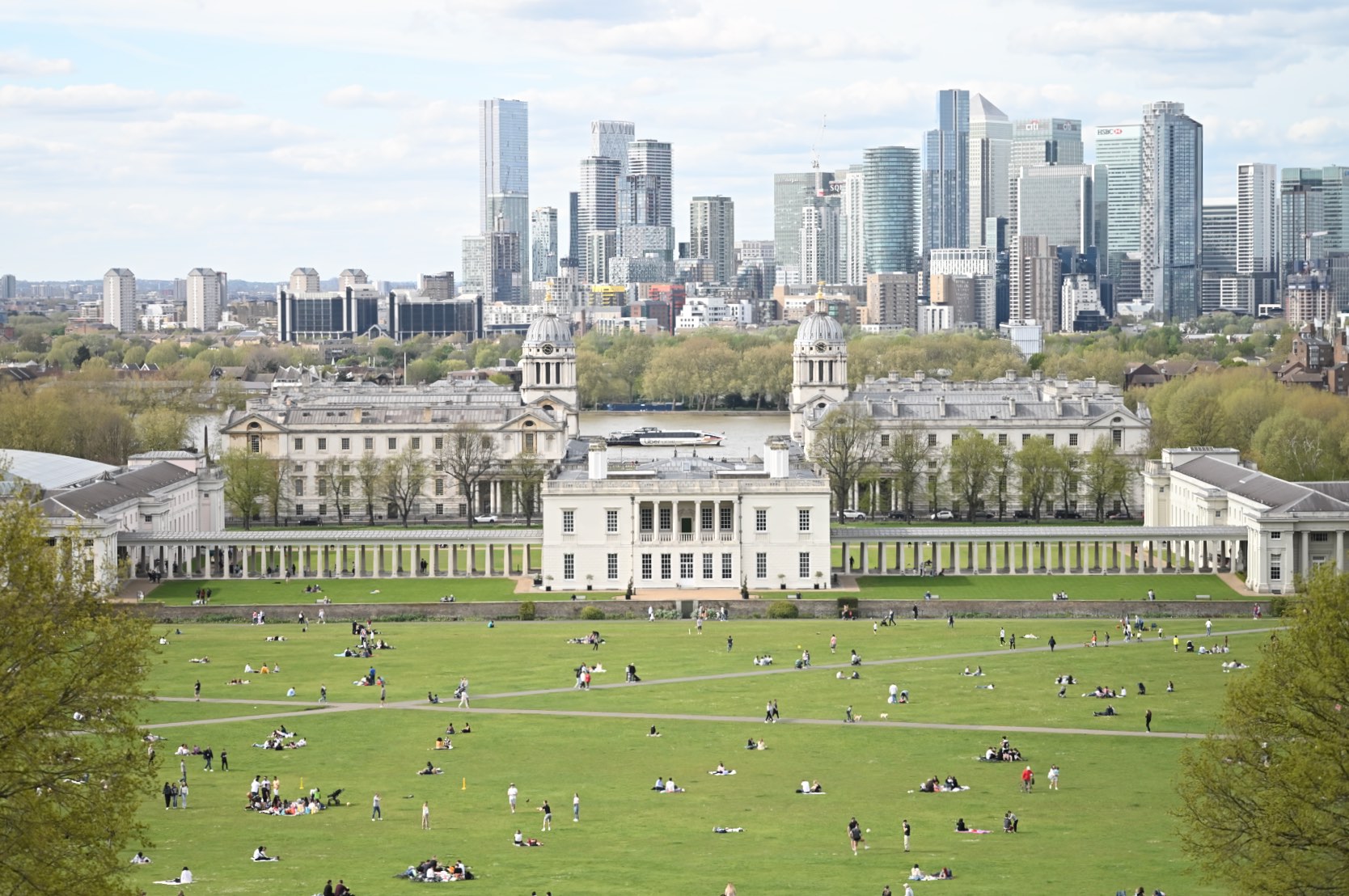
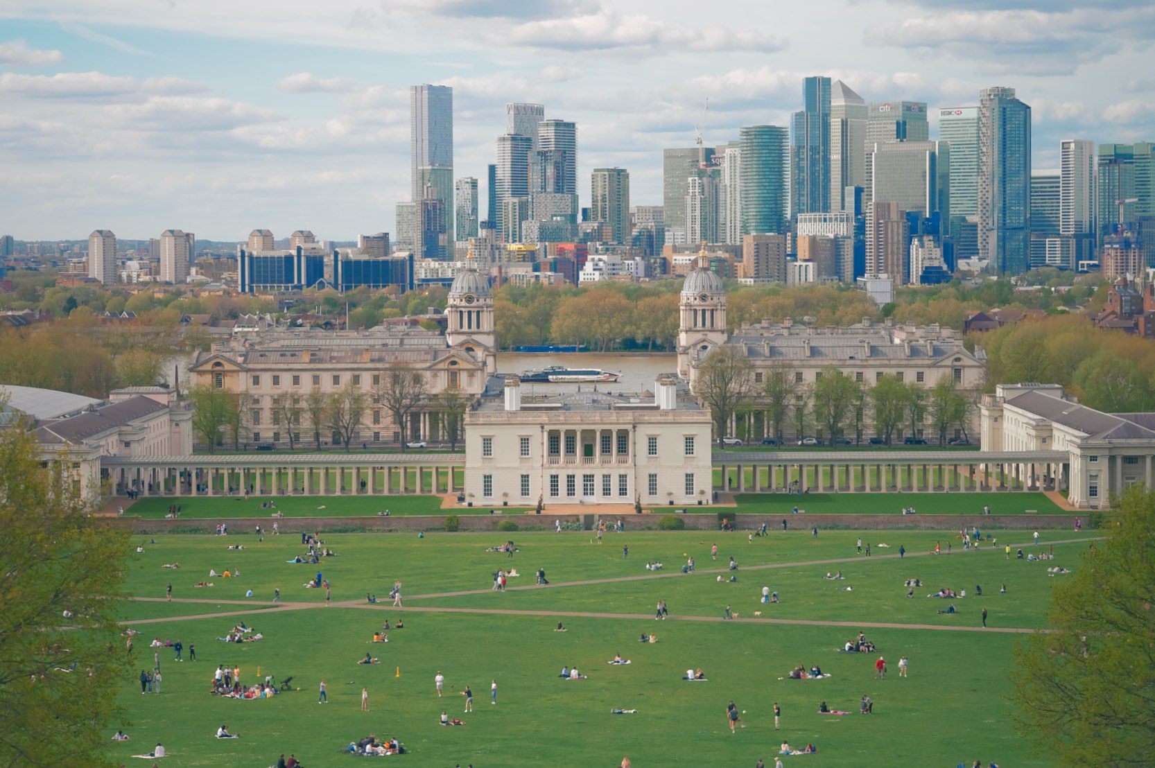
So let’s go back to the earlier shot:
Yes, that is the same shot as earlier. See the same people? They’re right there, on the left, in the distance. Yes, 24MP is a lot.
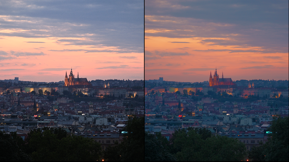
Anyway, that is rendered using Nikon’s “Standard” picture control. So what if…
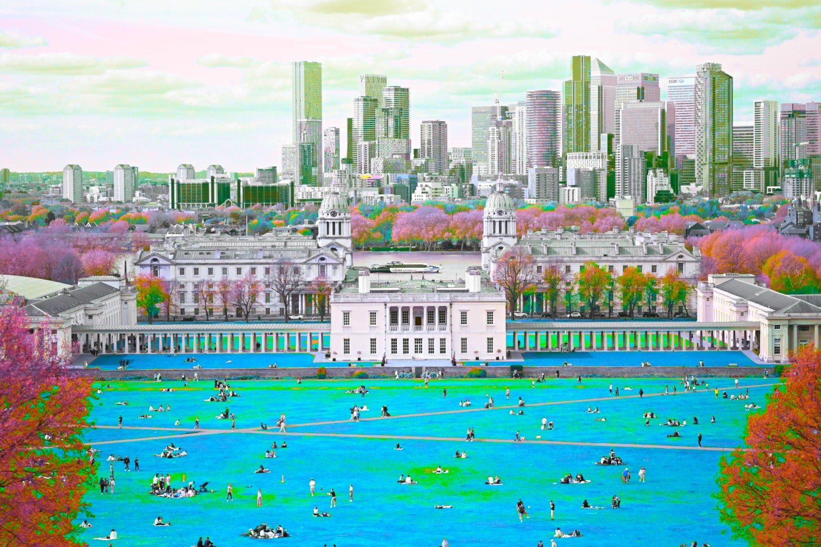
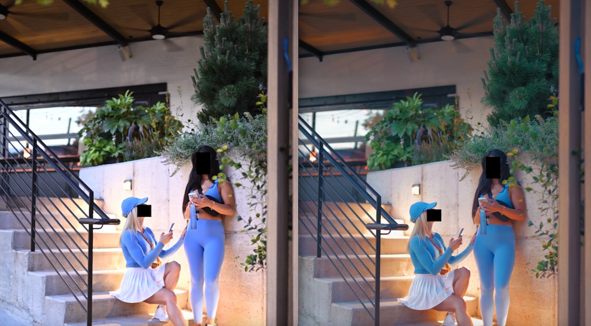
Oops, got a little carried away. But you get the point. I shifted bluer greens a tad toward cyan / blue; and yellower greens are subtly shifted slightly toward magenta, etc. This was using the new Flexible Picture Controls. And yes, that’s how it would render in-camera (with the raw retaining the full color data).
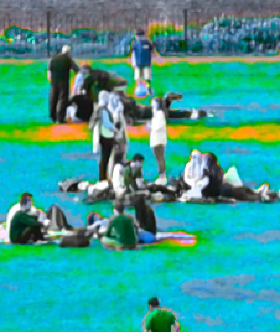
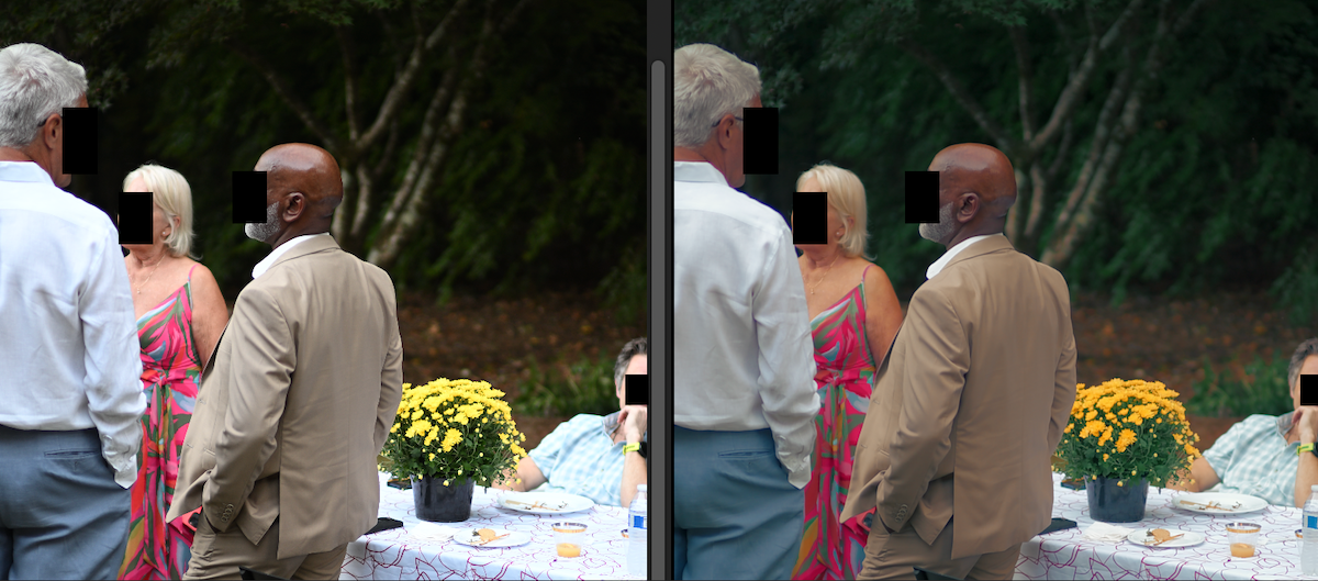
How’s our little family from earlier doing?
Oh. It appears they are being hunted by the infrared view of the Predator. I’m guessing he’ll spare the weak ones and only go after the strongest. Too bad it didn’t rain and get the ground all muddy so that they could mask themselves, set traps, and inspire Home Alone. Oh well. C’est la vie. Fun fact about Jean Claude Van Damme…
Anyway, I’ll start with a series of diverse images (diverse lighting, subjects, colors, etc.), create a base flexible picture control, tweak it over time, and retroactively apply to see how it will affect previous iterations. Because unlike with editing, the goal here isn’t to edit one-by-one–it’s to have a handful of profiles that just work for any image.
For example, there are some aesthetic things I liked about color response on various film stock (regardless of technical accuracy); but I don’t always like everything about film simulations.
Like some have terrible skin tones for darker people because they only designed the film for fair-skinned people. Or looking at greens on today’s cameras, they’ll sometimes look almost neon; while on some stock they might be be very saturated but also cooler and darker. I also like some tweaks like subtly accentuating how most lighting tends to be warm and shadows tend to be relatively cool. And I sometimes like a softer (rather than sharper and contrasty) look, along with smoother rolloffs, especially for highlights. And I also like pairing these specifically with my ZF & Voigtlander lenses, just to complete the experience and vibe.
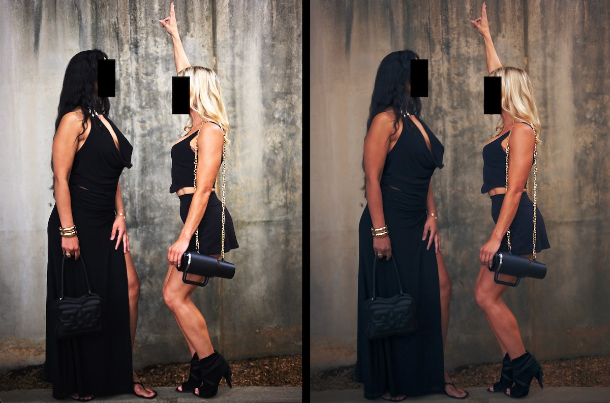
And so my main custom flexible picture control would render this same image from earlier instead like this:
Or here are just a handful of examples from this same picture control, side-by-side. These are really just to show differences in specific colors, in warmth in various tonal ranges, shadow/highlight rolloff, etc. Or just the overall vibe.
And then I might see that the magenta seems to be super saturated, and maybe I should dial that back. Or maybe it’s overall too flat and I should stretch out tones. Or maybe I like that because it reminds me of a printed photo. Or make whichever other tweaks. See how that affects other images. See how it looks on a phone. See how they print. Etc. Rinse, repeat.
And whether you like a retro/filmy vibe, a super contrasty grungy look, something artistic and abstract, or several different vibes for different scenarios, the key is: we have a lot of flexibility and control over the color science directly within the cameras now–far more than we already had with advanced picture controls. And far more than other brands offer. The one brand that often comes to mind is Fuji and their film simulations; but I’m confident I could recreate the film simulations of my XPro2 if I wanted to. And this just reminded me that I still have one of those somewhere…haven’t used it in a while; but my ZF + Voigtlander goes everywhere. (I wonder what the Fuji is worth…? Maybe I’ll sell it and get a ZR…)
Oh, and these work in video too! Including 10-bit h.265 video.
A lot of the conversation is often (for some reason) “what’s the dynamic range” or “how many megapixels?” But I hope Nikon continues development on features like this, with even more fine-tuned controls in the future. They’re fun and they can significantly alter the experience. And it’s too bad this isn’t in all of Nikon’s cameras. While the Zfc had a lot of built-in “filters,” I think it’s sad that it probably won’t get this until perhaps a Zfc-ii. But the ZF has it. Now in silver! Which I wish they had at launch.
TL;DR (the best place to put a TL;DR is always at the end): Color science is complex and has both scientific and artsy components. These flexible picture controls are brilliant. And since these cameras are powerful little supercomputers, they allow you to do a lot of color science experiments and just go out and shoot and share, outside of the editing room. If you just want to have fun shooting, you should be using these. Nikon’s color grade? A+
Almost forgot…I’m excited for the film grain simulation firmware!
– RC Jenkins, a formally educated, world-renowned expert in all subjects & internet user